Let’s face it. Machine Learning is the new fad. The big AI dream isn’t some distant dream anymore. So in this article, we’ll be going through something known as the “Principle of Maximum Likelihood ”. It’s a pretty simple principle to state, but the majority of learning algorithms in Machine Learning work because of this simple theorem.
What is it about ?
The principle of maximum likelihood is a method of obtaining the optimum values of the parameters that define a model. And while doing so, you increase the likelihood of your model reaching the “true ” model.
Okay. That probably made no sense. Let’s go through a simple example which illustrates the principle of maximum likelihood.
Now consider you have two coins; let’s call them A and B. Let the probability of getting a head with coin A be 0.5 and the probability of getting a head with coin B be 0.8. Now, let’s play a game. I randomly picked one of the two coins, tossed it three times and got 3 heads. Your job is to tell me which coin I picked.
Of course, this sounds trivial as coin B has a higher chances of landing heads. But let’s see how we would define our problem mathematically. So, we got three heads.


Now, since the tossing of coins is an independent event, i.e., the outcome of the first toss does not affect the outcome of the second toss, I can simplify the above equation as,


Applications in Machine Learning
Let’s now see how the principle of maximum likelihood could be applied in Machine Learning. We will be looking at two of the most fundamental supervised Machine Learning algorithms.
Consider the following example. You are given a dataset that contains the areas of houses and the prices at which those houses were purchased. That is, you have a dataset in which each entry is of the form (area, price). Now suppose you were given the area of a new house, a house that does not belong in your dataset, how would you predict the price of the house? This is done with linear regression.
But now, suppose your dataset contained the areas of houses along with a label of the house, which takes the value “0” if the house is “small” or “1” if the house is “large” (well… seems like a rather trivial task… But let’s convince ourselves that this is a rather difficult task for now). So, this kind of classification is what Logistic Regression is good for.
Linear Regression
As we just discussed, linear regression is a method of predicting future / new values given an existing dataset from which we can learn something about the correlation between different variables (in the above example, the correlation between area and price). How does it work ? Consider the following example.
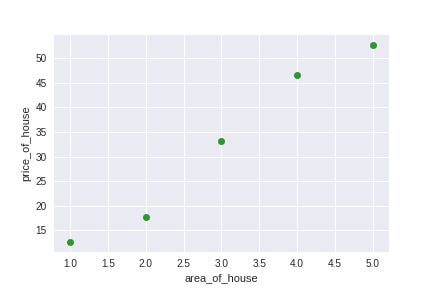
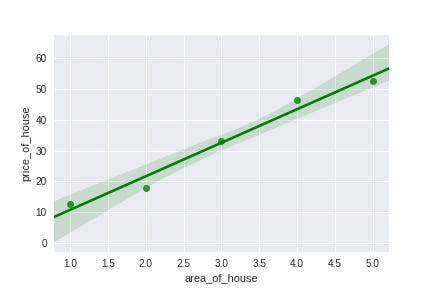
Given a set of pair-values (x,y), our objective is to find a function f which maps x to y as accurately as possible .That is, given the area of a new house, we need to accurately predict the price of the house. Let’s try plotting our dataset with house_area on the X axis and price on the Y axis.

We will now describe our cost function a bit more formally. Since our cost function is the error between the prediction our model makes and the actual price of the house, we will write our cost function as

( Please note. The 1/(2n) factor is just to make the math a bit more neat. It does not affect the convex nature ( the shape ) of the cost function in any manner. So minimizing J(m,c)*k where k is some constant and obtaining the optimum values of m and c is the same as minimizing J(m,c) and obtaining m,c)
So, how do we minimize this error? Simple. Find the partial derivative of J with respect to m and the partial derivative of J with respect to c and minimize J. You could do this by gradient descent, Newton-Raphson’s or some other algorithm.

But now the question arises: How can you be so sure that minimizing the above function will always give you the best possible parameters? That is, how can you say for sure that regardless what dataset you use, you will always arrive at the best possible values of the parameters by using the above function as your cost function ?
Let’s try defining our regression problem in a slightly different way. Now consider our earlier dataset.
Firstly, let’s assume that each of our (area_house,price_of_house) entry in our dataset is independent of each other (that is, the price of one house has nothing to do with the price of another house)
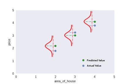
Secondly, I’m going to go ahead and assume that each entry in my dataset comes from a normal distribution centered at the prediction I make with a model and some constant standard deviation. That is; for actual_price1, I’m going to assume that it comes from a normal distribution with a mean of predicted_price1 with standard-deviation sigma. Similarly, actual_price2 comes from a distribution with mean of predicted_price2 and standard-deviation sigma and so on…


Now because of my Assumption, I can write the above expression as


Now, you might be wondering, all of this is based on the two assumptions I made above. How can you be certain that the assumptions hold for each and every dataset you work with ? Well… you can’t. Although both the assumptions hold true for most the cases ( the second assumption due to the Central Limit Theorem and the first assumption simply because your entries are often independent of each other ), there can definitely be cases where these assumptions can be violated. So, some initial investigation into your data is always necessary before you can start running other machine learning algorithms on your dataset.
Conclusion
Well.. That brings us to the end of the part 1! In the next part, we’ll be going through how the principle of maximum likelihood can be applied to find the cost function of Logistic Regression.